Methods
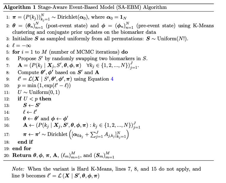
SA-EBM Algorithm
Graphic Model

Important Notice: Corrections have been made to Conjugate Priors, Experiment 9, and ADNI Results. Please review the updated sections for details.
As diseases progress, they increasingly impact more cognitive and biological factors.
By formulating probabilistic models with this basic assumption, Event-Based Models (EBMs) enable researchers
to discover the progression of a disease that makes earlier diagnosis and effective clinical interventions possible.
We build on prior EBMs with two major improvements: (1) dynamic estimation of healthy and pathological biomarker distributions,
and (2) explicit modeling of disease stage distribution. We tested existing approaches and our novel approach on 9,000 synthetic datasets and also the real-world ADNI data.
We found that our stage-aware EBM (SA-EBM) significantly outperforms prior methods,
such as Gaussian Mixture Model (GMM) EBM, Kernel Density Estimation EBM and Discriminative EBM,
in accurately recovering the order of disease events and assigning individual disease stages.
Our Python package can be installed by pip install pysaebm.
| ID | Impacted | FUS-FCI | P-Tau | MMSE | AB | HIP-FCI | PCC-FCI | … |
|---|---|---|---|---|---|---|---|---|
| 1 | Yes | 27.16 | -6.14 | 24.49 | 147.99 | 1.59 | 2.80 | … |
| 2 | Yes | 17.20 | 57.89 | 24.43 | 157.13 | -4.06 | 8.84 | … |
| 3 | Yes | 13.99 | 62.51 | 20.87 | 158.12 | 6.48 | 4.42 | … |
| 4 | No | 3.38 | 26.23 | 27.05 | 275.64 | -2.94 | 10.68 | … |
| 5 | No | 9.90 | 20.60 | 28.97 | 242.11 | -2.81 | 5.69 | … |
| 6 | No | 9.29 | 40.00 | 26.53 | 343.85 | -3.56 | 7.31 | … |
| ⋮ | ⋮ | ⋮ | ⋮ | ⋮ | ⋮ | ⋮ | ⋮ | ⋱ |
This table represents a typical cross-sectional dataset containing biomarker measurements from both healthy and progressing participants. The challenge is to infer the temporal sequence in which biomarkers become pathological as the disease develops. This table clearly illustrates that the task is daunting without the support of advanced statistical models.
In Appendix B.2 of the paper, we originally wrote that “$m_n$ and $s_n^2$ are the resulting posterior estimates.” To clarify: $m_n, n_n, v_n, s_n^2$ are the updated hyperparameters of the Normal–Inverse–Gamma posterior.
In our implementation, we use the posterior mean of $\mu$, which equals $m_n$, and the posterior mean of $\sigma^2$ under the corresponding Inverse–Gamma distribution, computed as
\[ \hat{\sigma}^2 = \frac{\beta_n}{\alpha_n - 1}, \quad \alpha_n = \tfrac{v_n}{2}, \;\; \beta_n = \tfrac{v_n s_n^2}{2}. \]
We then report $\hat{\sigma} = \sqrt{\hat{\sigma}^2}$ as the posterior standard deviation.
This clarification does not affect any reported results, but ensures consistency between the mathematical description and the implementation.

Average normalized Kendall's Tau distance values (± 95% CI). Each panel represents a different experimental configuration with varying data generation models, stage distributions, and biomarker distributions.
The X-axis within each panel shows different participant sizes (J = 50, 200, 500, 1000). Within each participant size are different healthy ratios (r), i.e., the percentage of healthy participants among all subjects. From left to right are r = 0.1, 0.25, 0.5, 0.75, 0.9.
The Y-axis shows the normalized Kendall's Tau distance (lower is better). Data points represent mean performance across 50 variants of the same experimental configuration, sample size, and healthy ratio. SA-EBM (Conjugate Priors) consistently outperform static and baseline methods. Performance generally improves with increasing sample size, while fixed-parameter methods degrade under high healthy ratios and non-Gaussian data.

Mean average errors (± 95% CI) for staging accuracy across nine synthetic experiments. Results are organized in the same way as in the above figure. SA-EBM outperforms static methods in staging accuracy.
Note that for the staging task, we only used the $\theta$ and $\phi$ parameters obtained from the inference stage and we do not assume knowledge of the diagnosis label (AD or CN). We did not use any prior or posteriors of stage stages obtained from the inference stage.

These Kendall's tau results include those of all SA-EBM variants.

These MAE results include those of all SA-EBM variants.
In the implementation of Experiment 9, the noise standard deviation was set to the square root of N * 0.05 instead of N * 0.05. This error increased the noise standard deviation from 0.50 to 0.71, resulting in larger noise. However, this does not impact the experiment's outcome. In fact, the increased noise likely undermines the performance of SA-EBM. That is to say, the performance of SA-EBM is expected to be better if using the correct implementation. This increased noises may benefit DEBM and DEBM GMM. However, given the current performance of benchmark algorithms in Experiment 9, it is unlikely that their performance would change significantly if the experiment were redone with the corrected implementation.
Due to this implementation error, the statement on page 9 of the paper, "N = 10 in our experiments ensured 95% of the noise fell within [−1, +1]," should be revised to: "N = 10 in our experiments ensured 95.5% of the noise fell within [−1.4, +1.4]."
Intracranial volume (ICV) normalization was not applied to brain volumes in the ADNI dataset, as it is standard practice due to natural variations in brain size. However, applying normalization altered the ADNI results, leading to new interpretations.
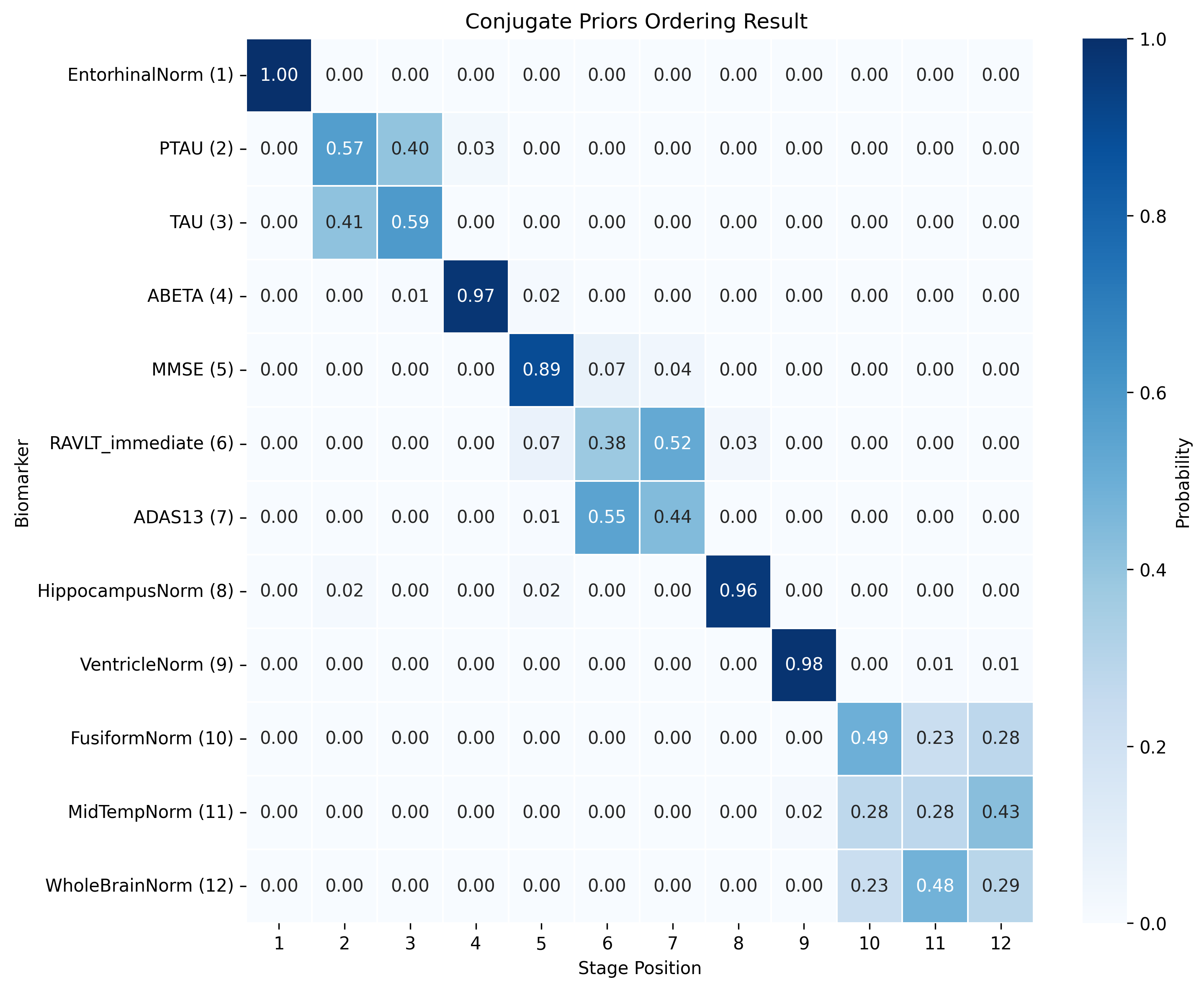
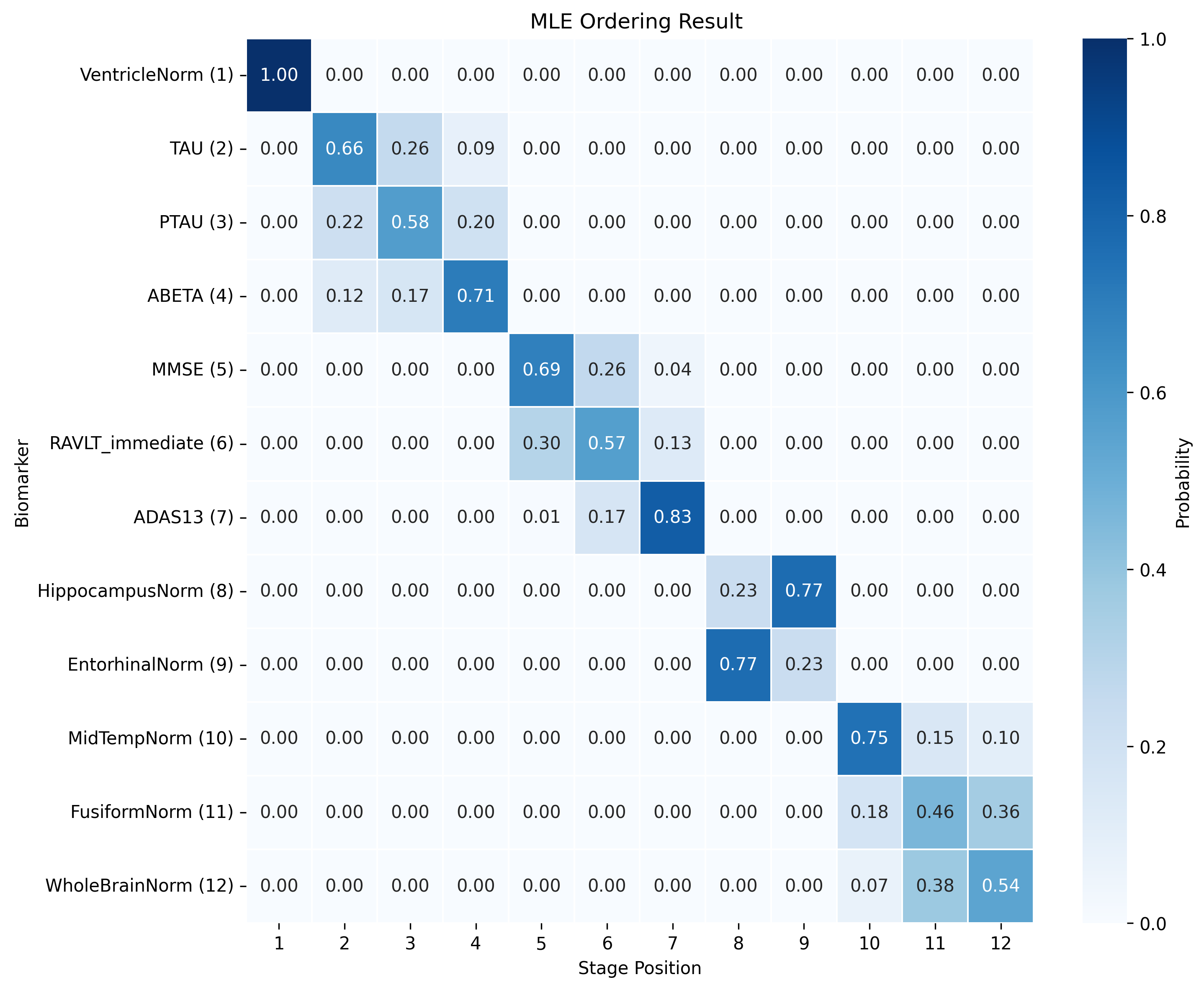
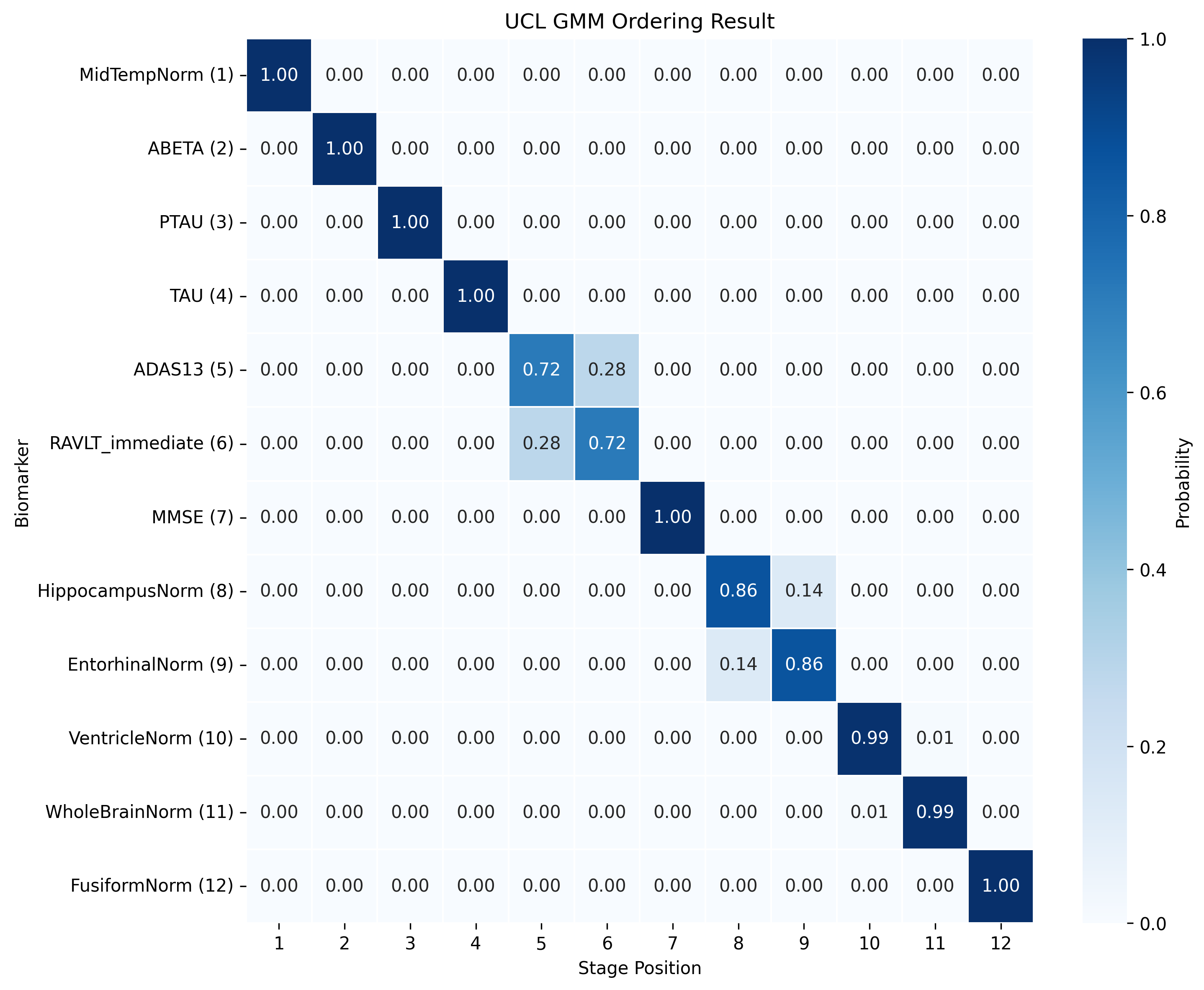
We tried ten random seeds for Conjugate Priors and UCL GMM to maximize the data log likelihood. For details, refer to https://github.com/hongtaoh/saebm?tab=readme-ov-file#adni.
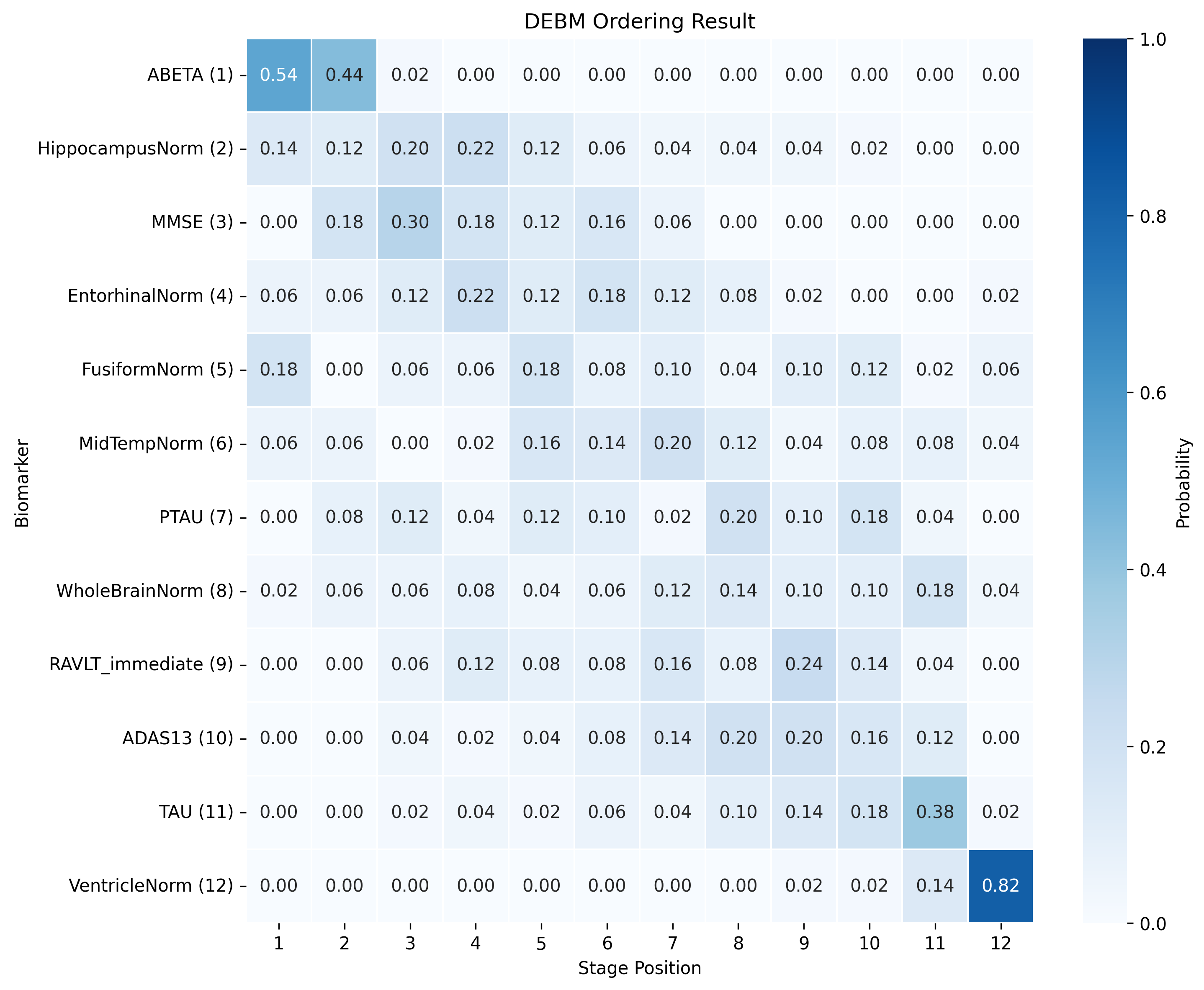
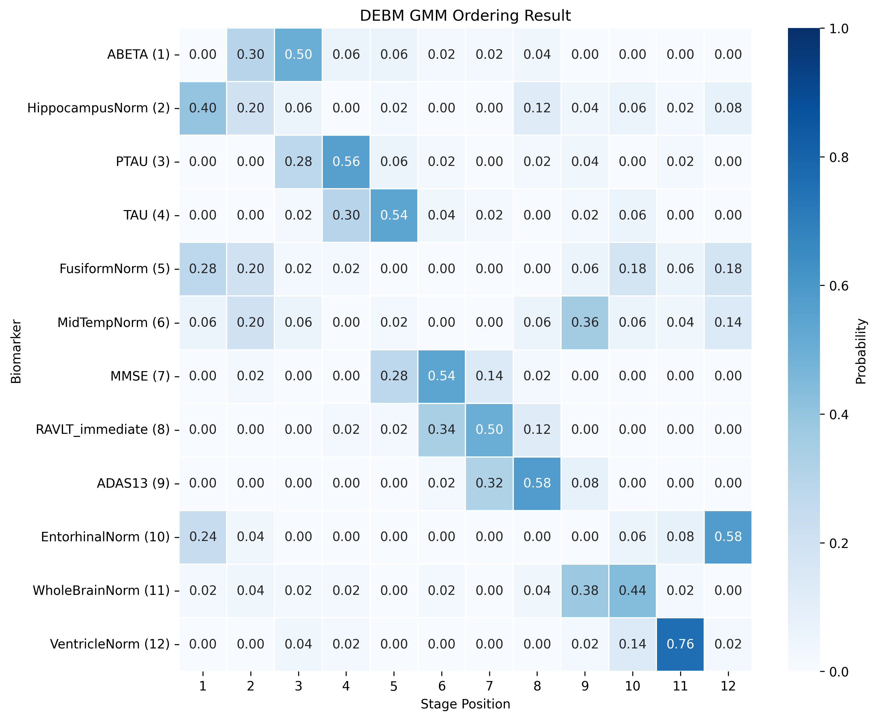
The DEBM model does not exhibit strong clustering, as similar biomarkers do not become pathological at similar times. DEBM GMM clustering performs better, but MRI brain volumes are scattered across the entire range. In contrast, UCL GMM, MLE, and Conjugate Priors demonstrate robust clustering. These models indicate that amyloid-beta (Aβ) and tau/p-tau become pathological before cognitive decline, followed by brain atrophy.
SA-EBM accurately assigns control and early mild cognitive impairment (EMCI) participants to early stages and Alzheimer’s disease (AD) participants to late stages. DEBM GMM fails to assign most healthy participants to stage 0 and places more healthy and EMCI participants in late stages. UCL GMM performs relatively well in the ADNI staging task but assigns an excessive number of EMCI participants to late stages.


@article{hao2025saebm,
      author    = {Hao, Hongtao and Prabhakaran, Vivek and Nair, Veena A and Adluru, Nagesh and Austerweil, Joseph L. and for the Alzheimer’s Disease Neuroimaging Initiative},
      title     = {Stage-Aware Event-Based Modeling (SA-EBM) for Disease Progression},
      journal   = {Machine Learning for Healthcare},
      year      = {2025},
    }